An example of reliability models: digraphs
The figures are in french and we apologize for the inconvenience, we will hopefully upload english figures as soon as possible.
1. Introduction
Digraphs represent a kind of graphical reliability models fallen in oblivion during the last decade. However, they have many advantages such as the possibility of seizing compact Boolean models; in addition, if we compare them to the fault trees, they are more expressive and can model closed-loop systems. Furthermore, they are effortlessly transformable in dynamic models and offer the same performance as BDMP (Boolean logic Driven Markov Processes), or to transform them in Bayesian networks in order to obtain a powerful diagnosis tool.
2. Digraphs' definitions
Digraphs are the generic term representing directed graphs and design a kind of reliability model. Nevertheless, there are two families of digraphs' definitions that induce an ambiguity in their meaning. In the remainder of this page, we will set the focus only on the second definition of digraphs with the mention of "Boolean", because it provide formal representation with a clear mathematical view.
2.1 Multi-states digraphs
Multi-state digraphs informal definition: the graphical representation of a physical system's state variables shows qualitatively the influences between variables. More specifically, the graph is constituted by nodes that represent the variables of the modelled system and edges that represent influences between variables. The edges are associated with numerical values usually chosen in the set {-10, -1, 0, 1, 10} which meanings are respectively: strong negative influence, negative influence, zero influence, positive influence, strong positive influence. Each node can be in one state taken from the following set of the possible states {null, normal, low, high, very low, very strong}. The multi-state digraphs are used to model effects propagation due to changes (failure or incident) of state variables from their nominal function.
This type of models cannot be considered as formal as it is easy to construct digraphs, even for closed-loop systems, of which the interpretation is not defined. What about, for example, a variable that receives three positive weak influences and a strong negative one simultaneously?
Despite their imperfections, the multi-state digraphs can be used to build structured reflections when doing HAZOP. However, recent researches are interested once again in the multi-state digraphs in order to construct a diagnosis tool with the qualitative reasoning.
2.2 Boolean Digraphs
Boolean digraph informal Definition: Graph where each node represents a Boolean variable depending on the state of upstream nodes and on the variable representing the intrinsic state of the node as well. A Boolean digraph can be used to support failure probability calculations of the modelled system starting from the probabilities associated with the inherent failure states.
The example which is illustrated in Figure 1 is a Boolean digraph model of a small redundant pumping system. The circles represent failures that occur either by the failure propagation of one of the inputs or by an intrinsic failure. The rectangle represents AND function on its inputs.
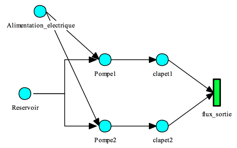
This digraph is a graphical representation of all the following Boolean equations (calling def (i) the intrinsic failure of the component 'i' and loss(i) the failure of the component 'i' from all causes:
Loss (out_flow) = Loss (valve1) AND Loss (valve2)
Loss (valve1) = def (valve1) OR Loss (Pump1)
Loss (valve2) = def (valve2) OR Loss (Pump2)
Loss (Pump1) = Loss (Power_supply) OR Loss (Tank) def OR (Pump1)
Loss (Pump2) = Loss (Power_supply) OR Loss (Tank) def OR (Pump2)
Loss (Power_supply) = def (Power_supply)
Loss (Tank = def (Tank)
It contains all failure Boolean functions specific to components that correspond to the gates of the fault tree in Figure 2.
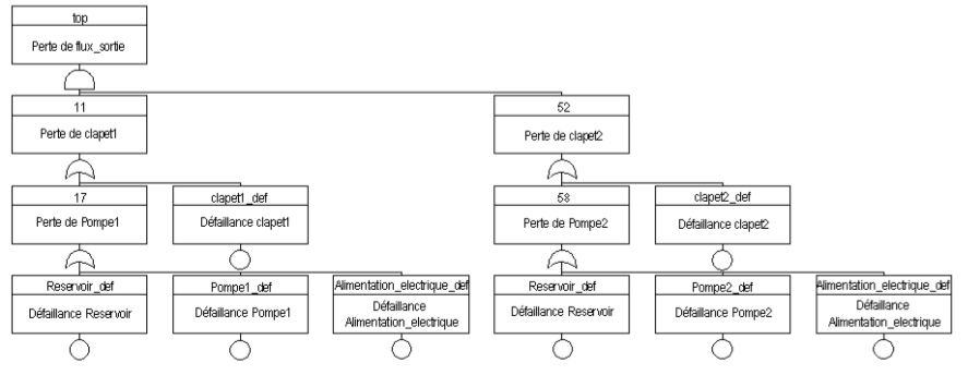
This simple example already shows advantages of digraphs: firstly, their representation is more compact and intuitive because in many situations (at least for systems whose main function is to transmit a flow step by step) the topology of digraphs is the projection of the physical system; secondly, they allow to model loop systems because they allow circuits, unlike fault trees. Nevertheless, allowing circuits necessarily requires some precautions and providing a formal definition is essential. It is also possible to perform various treatments on digraphs with a ATMS (Assumption Truth Maintenance System) based on BDD.
Boolean digraph formal definition: The directed graph (V, E) comprising a finite number of nodes V and a finite number of edges oriented E. Each node 'i' is associated with one or two Boolean variables. The variable loss (i) still exists and represents all kinds of failures (intrinsic or propagate) of component or system's function associated to 'i'. The variable def(i) the existence of which is still optional and represents an intrinsic failure mode. In addition, the node 'i' is associated with the following Boolean formula: Loss(i) = def(i) OR k_on_n (ki, loss(parent(i)); or simply: loss(i) = k_sur_n (ki, loss(parent(i)) weather def(i) exists.
In these expressions, loss(parent(i)) is an abuse of notation to denote the set of variables 'Loss' of parents of 'i' and k_sur_n (k, x) is a Boolean formula build on the literals 'xi' equal to 1 when the number of its arguments having the value 1 is at least equal to k. This formula generalizes the formulas AND and OR. The digraph can be used to support a probability calculation since it combines each intrinsic variable to stochastic process with values in {0, 1}. Indeed, each of Boolean functions are represented in the digraph becomes herself a stochastic process with values {0, 1} for which we can calculate reliability and availability. The simplest case is when we consider that the variables are initialized at 't = 0' according to a Bernoulli law and they keep their value indefinitely thereafter, because in this case the reliability is equal to availability and all results become independent on time.
3 Processing of classical digraphs
3.1 Preamble: notion of dual digraph
The fact that the topology of the digraph modelling a system is very similar to the system itself suggests that the digraph might as well model (in the manner of a reliability diagram) functioning flow propagation rather than flow failure propagation.
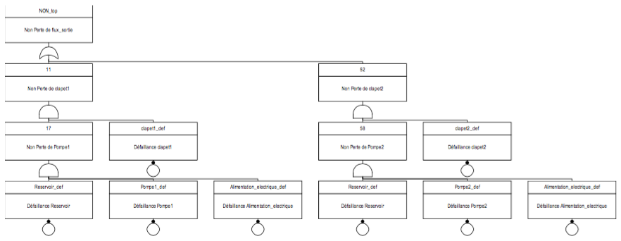
Actually, it is possible to pass from 'failure' digraph (that is to say, as we have described so far) to the 'good-functioning' one. To do so, we have to reverse all Boolean functions. Thus, without changing the design of the digraph of Figure 1
 , we can consider that it represents the success tree in Figure 3; itself is the dual tree of the tree in Figure 2
 . So failures become good functioning under the effect of the small black circles. Henceforth, the rectangles in good functioning digraph represent "OR" gates and the circles "AND" gates.
3.2 Unlooped Digraphs
Unlooped digraphs can be used by the methods that we describe in Section 3.3, but it will be more satisfying (for reasons of performance and features) to leverage their unlooped character and transform them into failure trees or Bayesian networks.
3.2.1 Transformation of digraphs into fault trees
The objective of this transformation is to use all the accumulated results from a half-century on the treatment fault trees. The automation of this transformation is trivial.We write the definition of the deducted variable from each node, depending on digraphs' structure, as it was done in Section 2.2 for the digraph of Figure 1
 . These equations represent a range of fault trees, of which the head events match the value 1 for the variable los (i). In order to obtain the Boolean function that links the basic variables def(k) to Loss(i), it suffices replacing each derived variable recursively by starting from Loss(i) and it is possible because of the lack of loops in the digraph.
To complete the description of the fault tree and make it quantitative, we simply combine models of stochastic processes def (k) variables since it is possible for the majority of fault trees computational tools. We can then make calculations of reliability, availability, and factors of importance in addition to determining the minimal cut.
3.2.2 Transformation of digraphs into Bayesian networks
It is now well known that the fault trees where basic events are associated with simple probabilities are a special case of Bayesian networks. Considering a fault trees as a Bayesian networks, we lose the concept of minimal cut and the possibility of purely qualitative treatment (no notion of probability), but we gain the opportunity to achieve the probabilistic diagnosis. It's the same thing for a digraph.
The first method is easier to explain, but its drawback is that it overloads the structure of Bayesian networks because it is necessary to have a node in Bayesian networks for each of its variable (either the type or the def loss). This method consists in associating with any node 'i' without parent node in digraph a probabilistic node of Bayesian networks that identifies def(i). Each node 'j' that has z set of parents will be associated with two nodes in Bayesian networks: the first probabilistic node match def(j) variable, and the second one is deterministic and corresponds to the variable loss(j). Figure 4 illustrate an example of the translation of the digraph in Figure 1
 into a Bayesian network. This figure was created using the Netica software, which displays the probabilities as percentages, where values are ranging from 0 to 100.
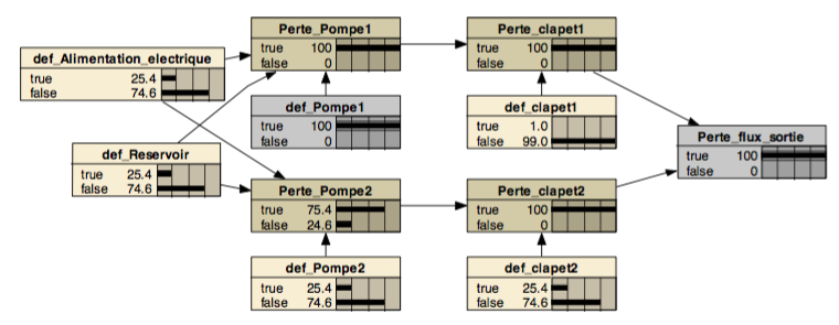
This figure shows an example of Bayesian network as a diagnostic tool. The state of the network displayed here corresponds to two observations: the output stream is lost and Pump1 is down. In this situation, we see that only the failure valve1 remains unlikely. To find out which component it would be more interesting to check, it is not possible to satisfying just by probabilistic arguments. Ideally, we should also have information about the cost of tests being performed on each component. Assuming known this information, it would be possible to use the methods such as MDP (Markov Decision Processes) to determine optimal diagnostic strategy and find the failures effortlessly.
The second method transforms the digraph in Bayesian network by giving a perfect isomorphic structure to that of the digraph, which then forces them to have all nodes in the probabilistic Bayesian network, the probability of intrinsic failure will be taken into account in the conditional probability tables. The tool Netica Bayesian networks, which was used to capture the Figure 4 allows an easy switching from the first representation to the second one, by absorbing the def_Pompe1,def_valve1, def_Pompe2 and def_valve2 nodes .
For example, Figure 6 illustrates the effect of absorption of def_valve1 node on the table of conditional probabilities that define Perte_valve1 node, passing from deterministic type (its value is known with certainty based on values his parents) to a probabilistic one (general nodes of Bayesian networks).


The second representation is certainly more compact and probably and have efficient computational side for large models, but it is less accurate, since it does not enter comments on the intrinsic state components. This is not necessarily a disadvantage because of the difficult task to obtain information on the intrinsic state of the components.
3.2.2 Transformation of digraphs into Relational models
The disadvantage in transforming digraphs into Bayesian networks as envisaged in the preceding section is that it requires creating different conditional probability for each item while the concept is still simple and repetitive using logic gates. However, PRM concepts, enhanced during the SKOOB project, provide a very efficient mean for modelling in order to gain more expressiveness in all abstraction levels.
You find here, some digraphs 'concepts described in a generic form O3prm language. The keywords of O3prm language are written in bold. Here below, we briefly describe the digraph of Figure 1
 in O3prm language.
interface Node{
	boolean loss;
}

class Leaf implements Node {
	boolean failure {[0.01, 0.99]};
	boolean loss = exist([def], true);
}

class OrNode extends Leaf {
	Node[] inputs;
	boolean loss = or([inputs.loss, failure]);
}

class AndNode implements Node {
	Node[] inputs;
	boolean loss = and([inputs.loss]);
}
In order to transform the digraph of Figure 1
 into PRM, we instantiate all its elements from the relational skeleton or classes level (see the following section : class inheritance). In this way and using some function of O3prm language such as "exists" and "forall", we avoid describing the conditional probability tables for all initiate items, so we save time.
system s {
	Leaf power_supply;
	Leaf tank;
	OrNode pump_1;
	pump_1.inputs += power_supply;
	pump_1.inputs += tank;
	OrNode valve1;
	valve_1.inputs += pump_1;
	OrNode pump_2;
	pump_2.inputs += power_supply;
	pump_2.inputs += tank;
	OrNode valve_2;
	valve_2.inputs += pump_2;
	AndNode out_flow;
	out_flow.inputs += valve1;
	out_flow.inputs += valve2;
}
5 Application example: cooling system
The software KB3 developed by EDF can achieve simply all discussed treatments in the sections above It was enough for it to develop a small "knowledge base" that embodies the concepts of dynamic digraphs. This knowledge base, called DigDyn and is part of the knowledge base available in open-source (on the site sourceforge.net) with the development tool of knowledge bases for KB3 called VisualFigaro.
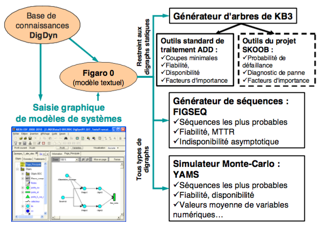
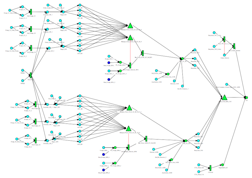
This knowledge base has to quickly study the reliability and availability of a repairable system 90 components incorporating passive redundancy. This system, modeled by the digraph of Figure 8 is the network cooling a data center. It helps maintain a constant temperature for a computer room hosting critical applications. It is composed of a double chilled water network and several production facilities in cold redundancy.
Here is an example of modelization of digraph with the PRM tools to make a PRM model
