
Semantics and definitions
1. Probabilistic Relational Model (PRM)
PRM is inspired by relational language, directly based on the BN and improved by object oriented paradigms, where the focus is set on classes of objects and by defining relations among these objects.
As we know, BN is not adequate for modelling large scale world; it quickly loses its expressivity due to the large number of the obtained variables, while PRM principle aims to gather these variables into clusters called classes. This new generic entity offers a flexible modelling framework when using object oriented programming.
This page provides precise definitions of the PRM semantics extended by the object oriented and supported by relational language.
1.1 The power surge example
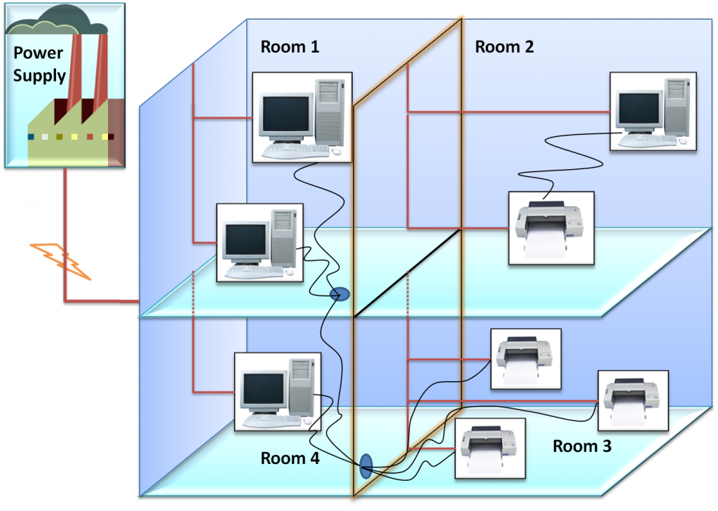
Power surge example is a computer maintenance problem where a set of computers and printers, located in different rooms, are powered by one or more power supplies. Breakdowns are caused by power surges, also known as voltage spikes. They can be caused by lightning strikes, power outages, tripped circuit breakers, short circuits, power transitions in other large equipment on the same power line, malfunctions caused by the Power Company, etc. Depending on the voltage spike intensity and the overall quality and age, electronic devices, i.e., computer and printer may breakdown after a power surge. Each equipment is described by its current state (state: {OK, NOK}). For computers, an additional attribute shows if we can print (canPrint: {can, cannot}). Finally, power supplies are described by their power state (power: {on, off, surge}), the surge state showing that at least one power surge occurred in the last 24 hours. Finally, a computer is usually plugged to one or more printers; it can print if at least one of its printers is functional.
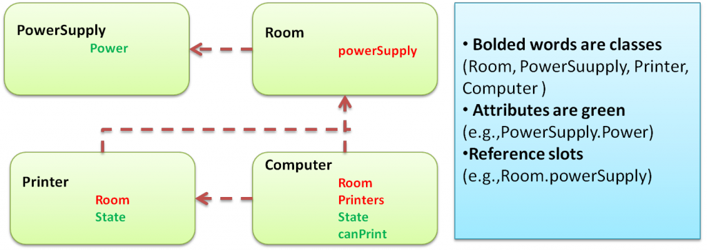
Relational schema below gives a simplistic view of PRM by illustrating relations between classes; each relation does not entail automatically a probabilistic dependency. However, this graph is the pattern to an infinite number of possible worlds.
2. PRM semantics definitions
2.1 Classe
The set of classes \(\chi={X_1,X_2,...,X_n}\) is the basic unit for the construction of PRM. Each class is associated with a set of attributes \(A(X)\) and a set of reference slots \(R(X)\). Classes are elaborate version of BN fragments.
2.2 Attributes
Attributes are encapsulated by classes. We denote \(X.A\) attribute of the class \(X\), e.g., Printer.state, and has a space of values \(Val(X.A)\). We precise that attributes at class level are generic patterns from which we create identical elementary entities that play the role of random variables in BN.
An Attribute \(X.A\) is represented by a triplet \(\langle\tau_{X.A} ,\pi(X.A),\phi_{X.A}\rangle\) where \(\tau_{X.A}\) is \(A.X\)'s type. \(\pi(X.A)\) is a set of attributes called parents of \(X.A\) and \(\phi_{X.A}\) a factor encoding the conditional probability distribution \(P(X.A|\pi(X.A))\).
-
\(\tau_{X.A}\) is an attribute’s type that describes a family of distinct discrete random variables sharing the same domain where \(\tau={l_1,...,l_n}\) and \(n\) is the domain size of \(\tau\). By defining attribute's type, we reduce the amount of redundant information that must be specified when modelling the system. This aspect will be presented later in class inheritance part.
-
Parents are attributes that impact the running attributes, e.g., Computer.state is the parent of Computer.canPrint.
-
In computer programming we consider attributes as local variable and those of BN as global ones.
2.3 Reference slots
Reference slots specify the conceptual relations that hold between classes. We use \(X.\rho\) to denote the reference slot \(\rho \in R(X)\) . \(\rho\) has a domain type \(domain(\rho)=X\) and a range type \(range(\rho)=Y\), where \(Y\) is a class in \(\chi\).
The inverse reference slot \(\rho^{-1}\) of \(\rho \in R(x)\) is the reference slot such that \(domain(\rho^{-1})=range(\rho)\) and \(range(\rho^{-1})=domain(\rho)\).
We use reference slots as pointers to access elements for a class to another, e.g., the reference slot Printer.room=Room is pointer towards the class Room such that we can access elements of the class Room through the class Printer.
Two kinds of reference slots can be distinguished: the first one is called simple if it defines a 1 to 1 relation, e.g., one computer is connected to one room, and the second one is called complex if it defines 1 to n relations, e.g., one room is connected to many computers; from the example we conclude that the inverse of simple reference slot is not always simple.
2.4 Slot chain
We denote by \(X.K\) a slot chain formed by a sequence of reference slots \({\rho_1,...,\rho_n}\) such that for all \(i\), \(range(\rho_i)=domain(\rho_{i+1})\). Slot chains are the practical use of reference slots to connect attributes from different classes together. E.g., Attribute Computer.state (respectively Printer.state) is connected to attribute PowerSupply.state through the slot chain Computer.room.power.state (respectively Printer.room.power.state).
The inverse slot chains are useful to retrieve attributes children defined in other classes. They are also slot chains obtained from a sequence of inverse reference slots \({\rho_{n}^{-1},...,\rho_{1}^{-1}}\) such that for all \(i\), \(range(\rho_{i+1}^{-1})=domain(\rho_{i}^{-1})\).
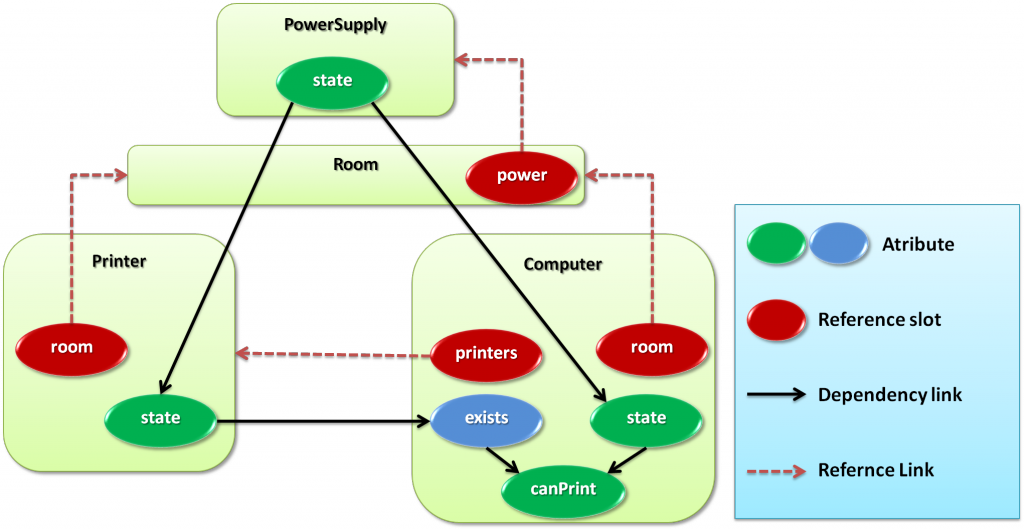
For example, in Figure 3 attribute PowerSupply.state has two children Printer.state and Computer.state that can be accessed using the inverse slot chains of Printer.room.power (denoted \(K\)) and Computer.room.power(denoted \(L\)):\(PowerSupply.K^{-1}.state\) and \(PowerSupply.L^{-1}.state\) respectively.
A slot chain is single if all its reference slots are single, otherwise it is multiple.
2.5 Output attribute
An output attribute \(X.A\) is an attribute such that there exists some attribute \(Y.B\) that is a child of \(X\) accessing \(X.A\) through a slot chain. We cannot define output attributes as attributes with children outside of their class, since such definition would discard recursive classes. Indeed, for such classes some attributes would access to attributes of their classes using a recursive reference slot and we would have \(X=Y\). Consequently, we must define an output attribute as an attribute being accessed using a slot chain.
3. Instantiation
We mean by instantiation the use of relational schemas for modelling a specific situation called word. This step of modelling allows us to pass from the generic class level to the instance level. Let \(I\) be an instance; from each class \(X\) we obtain a set of objects in \(I\) denoted \(I(X)\), e.g., from the class Room we obtain room1, room2 …etc . Each object has a set of attributes \(A(x)\) and a set of reference slots \(R(x)\). Attributes and reference slots of an object \(x\) are denoted by \(x.A\) and \(x.\rho\) respectively.
Attributes create BN fragments while reference slots refer to sets of their range’s instances. Thus, instantiated slot chains can be used to access instances attributes parents. Nevertheless, attributes represent distinct random variable only if they are at the instance level.
3.1 Relational skeleton
A relational skeleton \(\sigma_r\) is a partial specification of an instance of a relational schema since we know the number of objects of each class \(\sigma_r(X_i)\) and relation that holds between objects. However, objects' attributes values of are left unspecified.
Under uncertainty, the relational skeleton behaves in the same way as BN by factorizing a joint probability distribution. It also uses two components: dependency structure \(S\) that defines the probabilistic dependencies and the parameters \(\theta_s\) associated with it, where the parameters \(\theta_s\) are defined by CPTs (conditional probability tables).
Let’s consider a relational skeleton \(S\) that represents a possible instantiation of the Relational schema in the Figure 4. It contains a set of instantiations, i.e., we obtain objects from classes and links from reference slots, links that represent dependencies between objects (for any instance \(i\) of class \(X\) and any reference slot \(X.\rho=\epsilon\), there exists at least one instance \(j \in S\) such that \(j\) is an instance of \(\epsilon\) and \(j \in range(i.\rho))\).
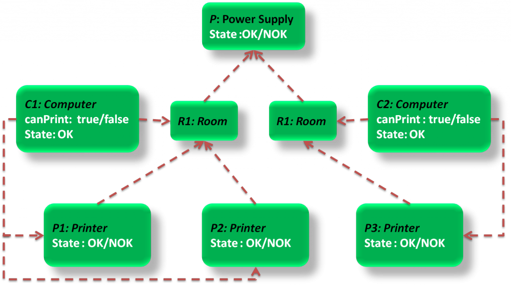
Indicate that two instances are connected by a reference slot)
3.2 Aggregate
Aggregators are attributes with a conditional probability distribution defined by a set of rules that can be used to generate the attribute’s CPT once it is instantiated and connected to its parents. They often allow to implement optimized data-structures preventing high memory consumptions.
Figure 3: Power surge model at the class level
Let us now give an overview: we denote by \(X.K\) the set of objects that are accessible through the slot chain \(K\) where \(K\) is complex. In order to define the probabilistic dependencies of \(X.A\) using the multi-set \({Y.B: Y \in Y.K}\), we consider an aggregate \(\gamma\) takes a multi-set of values of some ground type, and returns a summary of it in the form of a discrete multi-valued attribute. The type of the aggregate can be the same as that of its arguments. However, we allow other types as well, e.g., an aggregate that reports the size of the set (with an upper and lower bounds on the possible sizes). We allow \(X.A\) to have as a parent \(\gamma(X.K.B)\) ; the semantics is that for any \(x \in X\), \(x.A\) will depend on the value of \(\gamma(X.K.B)\).
Many aggregate functions could be used, e.g., min, max, for all, exist and k-gates...
4. PRM
We can define the PRM according to his two levels of abstraction as follows:
At the class level (generic level):
A PRM for a relational schema \(R\) is defined by a set of classes \(X \in \chi\). Each class \(X\) have a set of attributes \(A \in A(X)\) and a set of reference slots \(\rho \in R(X)\) knowing that:
-
A set of parents \(\pi (X.A)={U_1,...,U_l}\), where each \(U_i\) has the form \(X.B\) or \(\gamma(X.K.B)\), where \(K\) is a slot chain and \(\gamma\) is an aggregate.
-
A legal conditional probability distribution (CPD), \(P(X.A|\pi(X.A)\).
At the instance level:
A PRM is defined through the relational skeleton \(\sigma_r\) which is itself a set of instantiations, i.e., from classes we obtain objects and their attributes and from reference slots the links that represent dependency relationships between objects. Henceforth, we can build the ground BN of PRM and \(\sigma_r\):
-
There is a node of every object’s attribute \(x.A\) where \(x \in \sigma_r(X)\).
-
\(x.A\) probabilistically depends on parents of the form \(x.B\) or \(x.K.B\) if \(K\) is not single valued, then the parent is the aggregate \(\gamma (x.K.B)\).
-
The conditional probability distribution for \(x.A\) is a CPT generated from factors \(\phi_x.A\).
-
Since the ground BN is built, many algorithms are available for computing inference. (Inference in PRM)