Bayesian networks and uncertainties

1. Bayesian Network (BN)

Bayesian Networks (synonyms: Bayesian net, belief network, Bayesian model or probabilistic directed acyclic graphical model), nowadays are the best known tool for modelling systems through knowledge including uncertainty (Pearl (1988)). The exploitation of Bayesian nets is extended to many fields, mainly where decision support is needed; they are useful in medical, military, financial, robotic and other fields...

BN are able to represent probabilistic relations between objects, according to the two paradigms associated to probabilities: they can represent both subjective knowledge, and frequentist (i.e. based on the repetition of an experiment with an uncertain outcome) probabilities. They are based on Baye’s theorem (see below). Thomas Bayes (1702-1761) considered that probability is not a property intrinsic to event realization but it depends on the knowledge deriving from the realization context.

2. Bayes’ Theorem

The probability of two events $A$ and $B$ happening, $P(A)$ is the probability of $A$ times the probability of $B$ given that $A$ has occurred.

$$P(A \cap B)=P(A)P(B|A)~~~~~~(1)$$

On the other hand, the probability of $A$ and $B$ is also equal to the probability of $B$ times the probability of $A$ given $B$.

$$P(B \cap A)=P(B)P(A|B)~~~~~~(2)$$

Equating the two yields:

$$P(A)P(B|A)=P(B)P(A|B)~~~~~~(3)$$

$$P(A|B)=\frac {P(A)P(B|A)}{P(B)}~~~~~~(4)$$

Equation (4) is known as Bayes’ Theorem and is the basis of statistical inference.

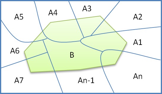
When the space $S$ (see figure 1) on which the probabilities are defined can be partitioned into a set of events $A_1, A_2...A_n$, the equation can be written also as follows:

$$P(B) = P(A_1 \cap B)+ P(A_2 \cap B) + ... + P(A_n \cap B)~~~~~~(5)$$

$$P(B) = P(B|A_1) P(A_1) + P(B|A_2) P(A_2)+... + P(B|A_n) P(A_n)~~~~~~(6)$$

$$P(A_i|B) = \frac{P(B | A_i) P(A_i)}{\sum_j P(B|A_j)P(A_j)}~~~~~~(7)$$

3. Inference

BN compute conditional probabilities of events knowing that statistical relationships may hold between them, this use is called inference. We introduce this concept through the simple example below.

3.1 Definition

BN is a graph, it contains nodes and edges: each node is associated with a set of probability tables and represents a random variable; each edge represents dependency between variables.

Let us model the following knowledge: «Both of Jeff and Paul work in the same company. Paul uses his car to go for his work while Jeff takes the train. Jeff rarely misses his train which is almost on time except when train strikes occur. However, a train strike does not necessarily imply that Jeff is late (in this case, Jeff can plan to take his car in the morning). A train strike can also delay Paul because of traffic congestion. But, the main reason that makes Paul late is that often he doesn’t hear the morning alarm. So, a train strike doesn’t significantly increase the probability of Paul’s delay.

If Jeff is delayed, we suppose that there is a train strike, and therefore Paul risks being late.
Let us suppose that Paul is late. This finding increases our belief in the two possible reasons for his delay (strike, alarm not heard). But if we learn that Jeff is late, we are tempted to conclude that a train strike is the main reason of their delay and the Alarm Problem doesn’t impact much our belief in Paul’s delay.

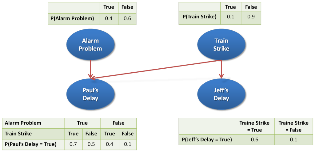
In this BN, nodes represent discrete random variables. In our example (see Figure 2), the four variables have only two states: 'True' and 'False'.

Edges represent statistical dependencies between variables. 'Train Strike' may impact ‘Jeff’s Delay'; we model this relationship by an edge from node 'Train Strike' to 'Jeff’s Delay'.

Each node considered as a random variable is associated to a table representing its joint probability distribution.

In fact, a Bayesian network is a concise representation of the joint probability distribution on all the random variables of the network. This probability distribution is the most complete information that we can have on all the considered random variables, and their inter-relations.

In this example, the joint probability distribution could be described by a table giving possible combinations of all the variables values.

3.2 Inference illustration

We are going now to take a closer look at how information flows within a BN's graph (see ). To explain simply, we are attempted to use our example.

Let us suggest the following case: We might want to calculate the probability of the event 'Jeff’s delay'.

P(Jeff’s Delay) = P(Jeff’s Delay | Train Strike) * P(Train Strike) + P(Jeff’s Delay | no Train Strike) * (1 - P(Train Strike)) = (0.6 * 0.1) + (0.1 * 0.9) = 0.15

This probability is an example of what we call a prior probability: it reflects our understanding of the event 'Jeffs Delay' where information of the other nodes state is absent.

The next table gathers the prior probabilities of all variables.

Alarm Problem	Train Strike	Jeff's Delay	Paul’s Delay
0.4	0.1	0.15	0.286

In fact, the most important use of Bayesian networks is to refresh variable probabilities when a new event is observed.

3.3 Examples

For example, we know that there is a strike. We can exploit this information in the model by P(Train Strike = True)=1. We derive directly from the table 'Jaff’s Delay' probability=0.6. Calculations show that the probability of 'Paul’s Delay'=0.52, and intuitively corresponds to “when Strike trains is on, Paul is less likely being late than Jeff”.
Let us suppose now that we do not know if there is a strike, but we know that Jeff is late. We can use the observation “Jeff’s delay=True” to refresh probabilities of 'Strike Train' and 'Paul’ Delay’. In fact, this new input significantly increases the probability that there is a strike (from 0.1 to 0.4), and slightly increases the probability that Paul is late (from 0.286 to 0.364).
Let us suppose that Paul is late. This finding increases our belief in two possible reasons of this delay (Train Strike and Alarm is not heard). In fact, the application of Bayes' theorem to calculate the refreshed 'Train Strike' probability is equal to 0.182 (knowing that the prior probability was equal to 0.1) and the refreshed probability of 'Paul’s delay’ probability is equal to 0.727 (knowing that the prior probability was equal to 0.4). In this case we bet on the second reason, What if we discovered that Jeff is also late. By entering this observation and applying Bayes' theorem, we find the refreshed probabilities: 0.571 for a 'Train Strike' and 0.637 for 'Paul’s Delay': this time, the two cases are almost equal.

This small example shows that the fact of using a simple model RB allows us to achieve a quantified deduction better than by using terms like "very likely" "unlikely", "increased slightly", etc...

4. Formal definitions

A Bayesian network can be formally defined by:

BN is a directed acyclic graph (DAG) $G$ , $G = G (X, E)$ where $X$ is the set of nodes of $G$ and $E$ the set of edges of $G$.
Let us consider $(\Omega,P)$ a finite probabilistic space
$A$ set of random variables associated with the nodes of the graph defined on $[\Omega,P]$ by :

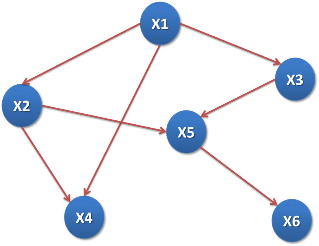
$P(X_1,X_2,\ldots,X_n)=\prod{P(X_i|C(X_i))}~~~~~~(8)$ With $C(X_i)$ is the set of parents of in the graph.

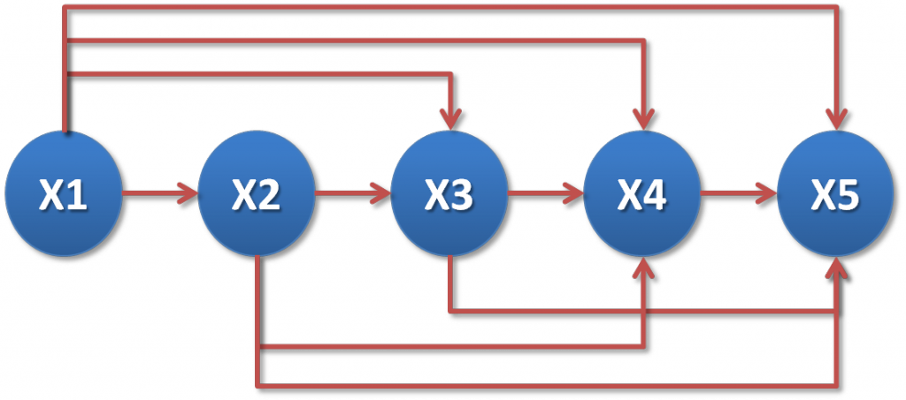
Any joint probability distribution can be represented by BN

Case of 5 variables: $X_1,X_2,X_3,X_4,X_5$ :

$$P(X_1,X_2,X_3,X_4,X_5)=P((((X_1,X_2),X_3),X_4),X_5)$$

$$=$$

$$P(X_5|X_1,X_2,X_3,X_4)P(X_4|X_1,X_2,X_3)P(X_3|X_1,X_2)P(X_2|X_1)P(X_1)~~~~~~(9)$$

Extreme case: if variables are globally independent, the graph contains no link at all
Calculation of probability: Factorization

$$P(X_1,X_2,X_3,X_4,X_5)$$

$$=$$

$$=$$

$$P(X_6 |X_5)P(X_5|X_2,X_3)P(X_4|X_1,X_2)P(X_3 |X_1)P(X_2 X_1)P(X_1)~~~~~~(10)$$

5. BN structures

In BN graph, three kinds of structure can be found:

5.1 Chains

5.2 Common parent

5.3 V-structures

6. D-separation

D-separation (D for dependence) determines whether a set of nodes $X$ is independent of another set $Y$, given a set of evidence nodes $Z$.

If every undirected path from a node in $X$ to a node in $Y$ is d-separated by $Z$. $X$ and $Y$ will be conditionally independent given $Z$.
A set of nodes $E$ d-separates two sets of nodes $X$ and $Y$ if every undirected path from a node in $X$ to a node in $Y$ is blocked given $E$.
A path $P$ is blocked given a set of nodes $B$ if there is a node $Z$ on the path for which one of three conditions holds:
1. $P$ contains a chain, $X$ ← $Z$ ←$Y$ such that the middle node $Z$ is in $B$.
2. $P$ contains a common parent, $X$← $Z$ → $Y$, such that the middle node $Z$ is in $B$.
3. $P$ contains a v-structure, $X$→ $Z$ ← $Y$, such that the middle node $Z$ is not in $B$ and no descendant of $Z$ is in $B$.

6.1 Example

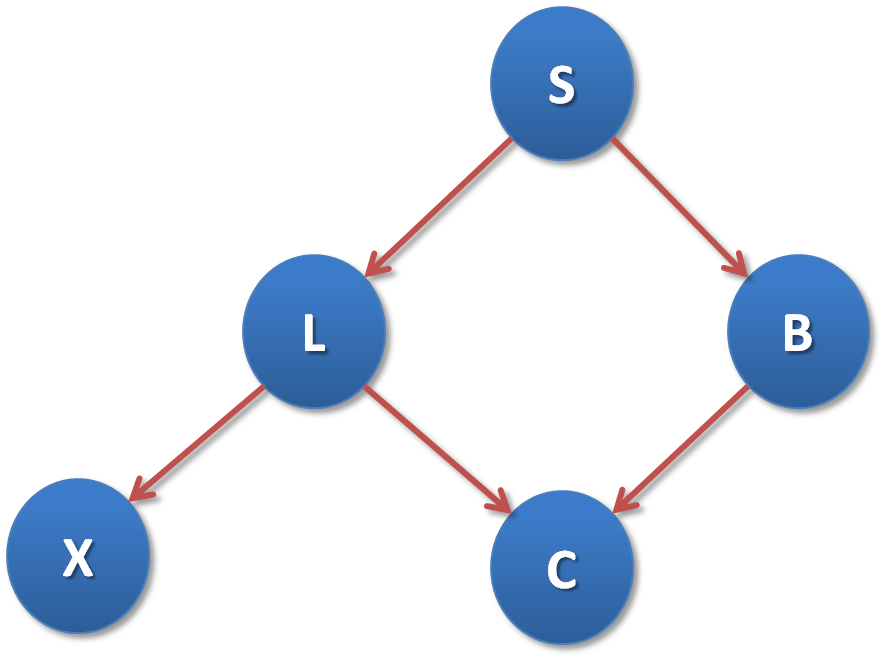
S: Smoker, L: Lung cancer, X: Positive X ray, C: Cough

$E$ is a set of evidence: $E = {B,C,L,S,X}$.

If the given evidence $E={S}$, the pairs $(L,B)$ and $(B,X)$ are d-separated given $S$.
If the given evidence $E={L}$, the pairs $(X,S)$, $(X,B)$ and $(X,C)$ are d-separated given $L$.
If the given evidence $E={S,E,B}$, the pairs $(C,S)$, $(C,X)$, $(X,C)$ are d-separated given the set ${L,B}$.

6.2 D-separation usefulness

D-separation helps to limit the probability calculations by using graph properties. If $X$ and $Y$ are d-separated by $Z$, and $Z$ is known. We suppose, moreover, that $P(X|Z)$ is computed. Finally, if new information about $Y$ is known, this result does not change our belief on $X$. So, we maintain the calculation of $P(X|Z)$ as the value of $P(X|Z,Y)$.

7. Conclusion

Bayesian networks are a powerful tool when it comes to modeling uncertainty. Currently, most real systems are classified complex due to their size and the interaction between their components, which means indeed, the necessity to build very large Bayesian networks. Thus, it makes it very difficult to build correct models and to perform inference because of combinatorial explosion. On this site we try to extend BN to other horizons, by using object oriented concepts combined with relational models and probabilistic models. This is what we call Open Object Oriented Probabilistic Relational Models (O3prm).

Risk Management

Bibliography

Judea Pearl. Probabilistic Reasoning in Intelligent Systems: Newtorks of Plausible Inference. Morgan Kaufmann Series in Representation and Reasoning. Morgan Kaufmann, 1988. ↩